Spectral Graph Theory - Scientific Computing with Python

Spectral Graph Theory studies graphs using associated matrices such as the adjacency matrix and graph Laplacian. Let $G(V, E)$ be a graph. We’ll let $n = |V|$ denote the number of vertices/nodes, and $m = |E|$ denote the number of edges. We’ll assume that vertices are indexed by $0,\dots,n-1$ , and edges are indexed by $0,\dots,m-1$ .

The adjacency matrix $A$ is a $n\times n$ matrix with $A_{i,j} = 1$ if $(i,j) \in E$ is an edge, and $A_{i,j} = 0$ if $(i,j) \notin E$ . If $G$ is an undirected graph, then $A$ is symmetric. If $G$ is directed, then $A$ need not be symmetric.

The degree of a node $i$ , $deg(i)$ is the number of neighbors of $i$ , meaning the number of edges which $i$ participates in. You can calculate the vector of degrees (a vector $d$ of length $n$ , where $d_i = deg(i)$ ), using matrix-vector mulpilication:

d = A 1

(1)

where 1 is the vector containing all 1s of length $n$ . You could also just sum the row entries of $A$ . We will also use $D = diag(d)$ - a diagonal matrix with $D_{i,i} = d_i$ .

The incidence matrix $B$ is a $n \times m$ matrix which encodes how edges and vertices are related. Let $e_k = (i,j)$ be an edge. Then the $k$ -th column of $B$ is all zeros except $B_{i,k} = -1$ , and $B_{j,k} = +1$ (for undirected graphs, it doesn’t matter which of $B_{i,k}$ and $B_{j,k}$ is +1 and which is -1 as long as they have opposite signs). Note that $B^T$ acts as a sort of difference operator on functions of vertices, meaning $B^T f$ is a vector of length $m$ which encodes the difference in fuction value over each edge.

You can check that $B^T 1_C = 0$ , where $1_C$ is a connected component indicator ( $1_C[i] = 1$ if $i \in C$ , and $1_C[i] = 0$ otherwise). $C\subseteq V$ is a connected component of the graph if all vertices in $C$ have a path between them, and there are no vertices in $V$ that are connected to $C$ which are not in $C$ . This implies $B^T 1 = 0$ .

The graph laplacian $L$ is an $n \times n$ matrix $L = D- A = B B^T$ . If the graph lies on a regular grid, then $L = -\Delta$ up to scaling by a finite difference width $h^2$ , but the graph laplacian is defined for all graphs.

Note that the nullspace of $L$ is the same as the nullspace of $B^T$ (the span of indicators on connected components).

In most cases, it makes sense to store all these matrices in sparse format.

import numpy as np
import scipy.linalg as la
import scipy.sparse as sparse
import scipy.sparse.linalg as sla
import matplotlib.pyplot as plt

import networkx as nx
from sklearn import metrics
from sklearn.cluster import KMeans

G = nx.gnp_random_graph(100, 0.1)
nx.draw(G)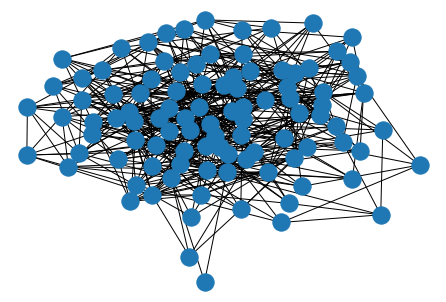

nx.adjacency_matrix(G)

<100x100 sparse matrix of type '<class 'numpy.int64'>'
	with 1006 stored elements in Compressed Sparse Row format>

nx.incidence_matrix(G)

<100x503 sparse matrix of type '<class 'numpy.float64'>'
	with 1006 stored elements in Compressed Sparse Column format>

nx.laplacian_matrix(G)

<100x100 sparse matrix of type '<class 'numpy.int64'>'
	with 1106 stored elements in Compressed Sparse Row format>

Exercise¶

For an undirected graph $G(V, E)$ , let $n = |V|$ and $m = |E|$ . Give an expression for the number of non-zeros in each of $A$ , $B$ , and $L$ in terms of $n$ and $m$ .

$A$ and $B$ both have $2m$ non-zeros. $L$ has $n + 2m$ non-zeros.

Random Walks on Graphs¶

In a random walk on a graph, we consider an agent who starts at a vertex $i$ , and then will chose a random neighbor of $i$ and “walk” along the connecting edge. Typically, we will consider taking a walk where a neighbor is chosen uniformly at random (i.e. with probability $1/d_i$ ). We’ll assume that every vertex of the graph has at least one neighbor so $D^{-1}$ makes sense.

This defines a Markov Chain with transition matrix $P = A D^{-1}$ (columns are scaled to 1). Note that even if $A$ is symmetric (for undirected graphs) that $P$ need not be symmetric because of the scaling by $D^{-1}$ .

The stationary distribution $x$ of the random walk is the top eigenvector of $P$ , is guaranteed to have eigenvalue 1, and is guaranteed to have non-negative entries. If we scale $x$ so $\|x\|_1 = 1$ , The entry $x_i$ can be interpreted as the probability that a random walker which has walked for a very large number of steps is at vertex $i$ .

Page Rank¶

PageRank is an early algorithm that was used to rank websites for search engines. The internet can be viewed as a directed graph of websites where there is a directed edge $(i, j)$ if webpage $j$ links to webpage $i$ . In this case, we compute the degree vector $d$ using the out-degree (counting the number of links out of a webpage). Then the transition matrix $P = A D^{-1}$ on the directed adjacency matrix defines a random walk on webpages where a user randomly clicks links to get from webpage to webpage. The idea is that more authoritative websites will have more links to them, so a random web surfer will be more likely to end up with them.

One of the issues with this model is that it is easy for a random walker to get “stuck” at a webpage with no out-going links. The idea of PageRank is to add a probability $\alpha$ that a web surfer will randomly go to another webpage which is not linked to by their current page. In this case, we can write the transition matrix

P = (1-\alpha) A D^{-1} + \frac{\alpha}{n} 11^T

(2)

We then calculate the stationary vector $x$ of this matrix. Websites with a larger entry in $x_i$ are deemed more authoritative.

Note that because $A$ is sparse, you’ll typically want to encode $\frac{1}{n}11^T$ as a linear operator (this takes the average of a vector, and broadcasts it to the appropriate shape). For internet-sized graphs this is a necessity.

Let’s look at the Les Miserables graph, which encodes interactions between characters in the novel Les Miserables by Victor Hugo.

G = nx.les_miserables_graph()
nx.draw_kamada_kawai(G)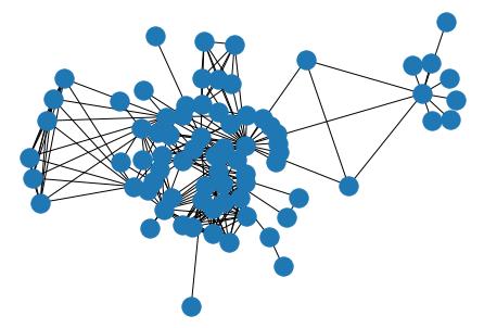

G.nodes(data=True)

NodeDataView({'Napoleon': {}, 'Myriel': {}, 'MlleBaptistine': {}, 'MmeMagloire': {}, 'CountessDeLo': {}, 'Geborand': {}, 'Champtercier': {}, 'Cravatte': {}, 'Count': {}, 'OldMan': {}, 'Valjean': {}, 'Labarre': {}, 'Marguerite': {}, 'MmeDeR': {}, 'Isabeau': {}, 'Gervais': {}, 'Listolier': {}, 'Tholomyes': {}, 'Fameuil': {}, 'Blacheville': {}, 'Favourite': {}, 'Dahlia': {}, 'Zephine': {}, 'Fantine': {}, 'MmeThenardier': {}, 'Thenardier': {}, 'Cosette': {}, 'Javert': {}, 'Fauchelevent': {}, 'Bamatabois': {}, 'Perpetue': {}, 'Simplice': {}, 'Scaufflaire': {}, 'Woman1': {}, 'Judge': {}, 'Champmathieu': {}, 'Brevet': {}, 'Chenildieu': {}, 'Cochepaille': {}, 'Pontmercy': {}, 'Boulatruelle': {}, 'Eponine': {}, 'Anzelma': {}, 'Woman2': {}, 'MotherInnocent': {}, 'Gribier': {}, 'MmeBurgon': {}, 'Jondrette': {}, 'Gavroche': {}, 'Gillenormand': {}, 'Magnon': {}, 'MlleGillenormand': {}, 'MmePontmercy': {}, 'MlleVaubois': {}, 'LtGillenormand': {}, 'Marius': {}, 'BaronessT': {}, 'Mabeuf': {}, 'Enjolras': {}, 'Combeferre': {}, 'Prouvaire': {}, 'Feuilly': {}, 'Courfeyrac': {}, 'Bahorel': {}, 'Bossuet': {}, 'Joly': {}, 'Grantaire': {}, 'MotherPlutarch': {}, 'Gueulemer': {}, 'Babet': {}, 'Claquesous': {}, 'Montparnasse': {}, 'Toussaint': {}, 'Child1': {}, 'Child2': {}, 'Brujon': {}, 'MmeHucheloup': {}})

A = nx.adjacency_matrix(G)
A

<77x77 sparse matrix of type '<class 'numpy.int64'>'
	with 508 stored elements in Compressed Sparse Row format>

n = A.shape[0]
d = A.sum(axis=1).reshape(1,-1) # compute degrees
Dinv = sparse.dia_matrix((1 / d, 0), shape=(n, n))
Dinv

<77x77 sparse matrix of type '<class 'numpy.float64'>'
	with 77 stored elements (1 diagonals) in DIAgonal format>

# works on square matrices or vectors
Onefun = lambda X : np.mean(X, axis=0).reshape(1,-1).repeat(X.shape[0], axis=0)

m = A.shape[0] # linear operator of shape of Adjacency matrix

OneOneT = sla.LinearOperator(
    shape   = (m,m),
    matvec  = Onefun,
    rmatvec = Onefun   
)

Let’s now construct the PageRank matrix and compute the top eigenpairs

alpha = 0.1

P = (1 - alpha) * sla.aslinearoperator(A @ Dinv) + alpha * OneOneT

lam, V = sla.eigs(P, k=5, which='LM')
lam

array([1.        +0.j, 0.83936036+0.j, 0.79746166+0.j, 0.74936377+0.j,
       0.70144813+0.j])

1j**2 == -1

True

x = np.abs(np.real(V[:,0])) # PageRank Vector
x

array([0.0133386 , 0.20399851, 0.0949893 , 0.10668613, 0.0133386 ,
       0.0133386 , 0.0133386 , 0.0133386 , 0.01926114, 0.0133386 ,
       0.57767244, 0.0107066 , 0.01679025, 0.0107066 , 0.0107066 ,
       0.0107066 , 0.07701289, 0.08277018, 0.07701289, 0.07992839,
       0.08300515, 0.08007966, 0.07716337, 0.15885074, 0.11720935,
       0.20909641, 0.22214954, 0.1583424 , 0.06719718, 0.04831427,
       0.01895798, 0.0377782 , 0.0107066 , 0.01702923, 0.06181196,
       0.06181196, 0.05030959, 0.05030959, 0.05030959, 0.02101082,
       0.01050109, 0.06584516, 0.02292668, 0.02325998, 0.02366606,
       0.0160557 , 0.02666986, 0.01541702, 0.1673304 , 0.104165  ,
       0.01375137, 0.09145499, 0.01729798, 0.01099474, 0.02347196,
       0.31496208, 0.0133744 , 0.05356893, 0.23233548, 0.16932592,
       0.05145195, 0.09653403, 0.21000629, 0.10143451, 0.16574335,
       0.1099175 , 0.04528474, 0.01645582, 0.08526568, 0.09150015,
       0.06900207, 0.04435378, 0.01961912, 0.02781421, 0.02781421,
       0.0472697 , 0.02410199])

i = np.argmax(x)
names = np.array([k for k, _ in G.nodes(data=True)])
names[i]

'Valjean'

perm = np.argsort(x)[::-1] # reverse sort
names[perm[:4]]

array(['Valjean', 'Marius', 'Enjolras', 'Cosette'], dtype='<U16')

The Graph Laplacian¶

Spectral Embeddings¶

Spectral embeddings are one way of obtaining locations of vertices of a graph for visualization. One way is to pretend that all edges are Hooke’s law springs, and to minimize the potential energy of a configuration of vertex locations subject to the constraint that we can’t have all points in the same location.

In one dimension:

\mathop{\mathsf{minimize}}_x \sum_{(i,j) \in E} (x_i - x_j)^2\\ \text{subject to } x^T 1 = 0, \|x\|_2 = 1

(3)

Note that the objective function is a quadratic form on the embedding vector $x$ :

\sum_{(i,j)\in E} (x_i - x_j)^2 = x^T B B^T x = x^T L x

(4)

Because the vector 1 is in the nullspace of $L$ , this is equivalent to finding the eigenvector with second-smallest eigenvalue.

For a higher-dimensional embedding, we can use the eigenvectors for the next-largest eigenvalues.

Attention: the first formula is not shown in the current notebook!

G = nx.grid_2d_graph(10,10)
L = nx.laplacian_matrix(G)
L = sparse.csr_matrix(L, dtype=np.float64)

lam, V = sla.eigsh(L, which='SM')
plt.scatter(V[:,1], V[:,2])
plt.show()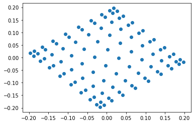

nx.draw_spectral(G)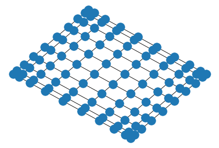

Spectral Clustering¶

Spectral clustering refers to using a spectral embedding to cluster nodes in a graph. Let $A, B \subset V$ with $A \cap B = \emptyset$ . We will denote

E(A, B) = \{(i,j) \in E \mid i\in A, j\in B\}

(5)

One way to try to find clusters is to attempt to find a set of nodes $S \subset V$ with $\bar{S} = V \setminus S$ , so that we minimize the cut objective

C(S) = \frac{|E(S, \bar{S})|}{\min \{|S|, |\bar{S}|\}}

(6)

The Cheeger inequality bounds the second-smallest eigenvalue of $L$ in terms of the optimal value of $C(S)$ . In fact, the way to construct a partition of the graph which is close to the optimal clustering minimizing $C(S)$ is to look at the eigenvector $x$ associated with the second smallest eigenvalue, and let $S = \{i \in V \mid x_i < 0\}$ .

As an example, let’s look at a graph generated by a stochastic block model with two clusters. The “ground-truth” clusters are the ground-truth communities in the model.

ns = [25, 25] # size of clusters
ps = [[0.3, 0.1], [0.1, 0.3]] # probability of edge
G = nx.stochastic_block_model(ns, ps)
true_clusters = [c for _, c in nx.get_node_attributes(G, 'block').items()]


nx.draw_kamada_kawai(G, with_labels=False, node_color=true_clusters)
plt.title("SBM with ground-truth clusters")
plt.show()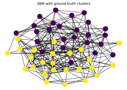

Now, let’s use spectral clustering to partition into two clusters

lam, V = sla.eigsh(nx.laplacian_matrix(G).astype(np.float64), which='SM')
x = V[:,1]
cs = x < 0 # get clusters

nx.draw_kamada_kawai(G, with_labels=False, node_color=cs)
plt.title("SBM with spectral clusters")
plt.show()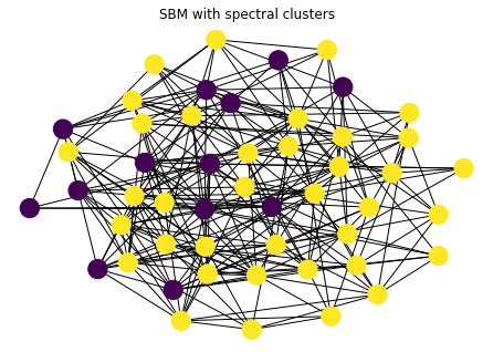

We’ll use the adjusted rand index to measure the quality of the clustering we obtained. A value of 1 means that we found the true clusters.

from sklearn import metrics

metrics.adjusted_rand_score(true_clusters, cs)

-0.014331210191082872

In general, you should use a dimension $d$ embedding when looking for $d+1$ clusters (so we used a dimension 1 embedding for 2 clusters). Let’s look at 4 clusters in a SBM

nclusters = 4
ns = [25 for i in range(nclusters)] # size of clusters
ps = 0.02 * np.ones((nclusters, nclusters)) + 0.25 * np.eye(nclusters)
G = nx.stochastic_block_model(ns, ps)
true_clusters = [c for _, c in nx.get_node_attributes(G, 'block').items()]

nx.draw_circular(G, with_labels=False, node_color=true_clusters)
plt.title("SBM with ground-truth clusters")
plt.show()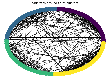

we’ll use K-means clustering in scikit learn to assign clusters.

from sklearn.cluster import KMeans

lam, V = sla.eigsh(nx.laplacian_matrix(G).astype(np.float64), k=nclusters+1, which='SM')
X = V[:,1:]
cs = KMeans(n_clusters=nclusters).fit_predict(X) # get clusters

nx.draw_circular(G, with_labels=False, node_color=cs)
plt.title("SBM with spectral clusters")
plt.show()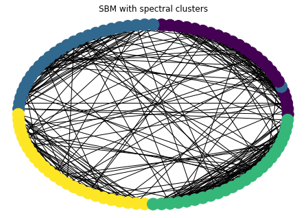

metrics.adjusted_rand_score(true_clusters, cs)

0.97305763367046

Exercise¶

We’ll consider the stochastic block model with $k=5$ clusters and $n=25$ nodes per cluster.

Let $p$ be denote the probability of an edge between nodes in the same cluster, and $q$ denote the probability of an edge between nodes in different clusters.

Plot a phase diagram of the adjusted rand index (ARI) score as $p$ and $q$ both vary in the range $[0,1]$