Convolutions and Fourier Transforms - Scientific Computing with Python

A convolution is a linear operator of the form

(f \ast g)(t) = \int f(\tau) g(t - \tau ) d\tau

(1)

In a discrete space, this turns into a sum

\sum_\tau f(\tau) g(t - \tau)

(2)

Convolutions are shift invariant, or time invariant. They frequently appear in temporal and spatial image processing, as well as in probability.

If we want to represent the discrete convolution operator as a matrix, we get a toeplitz matrix $G$

G = \begin{bmatrix} g(0) & g(1) & g(2) & \dots\\ g(-1) & g(0) & g(1) &\dots\\ g(-2) & g(-1) & g(0) & \dots\\ \vdots & & &\ddots \end{bmatrix}

(3)

A circulant matrix acting on a discrete signal of length $N$ is a toeplitz matrix where $g(-i) = g(N-i)$ .

import numpy as np
import scipy as sp
import scipy.linalg as la
from scipy import ndimage
from scipy.fft import dct, dctn, fft, idct, idctn, ifft
import matplotlib.pyplot as plt

from numba import njit
import skimage
import torch

c = np.arange(0,-4, -1) # first column
r = np.arange(4) # first row
la.toeplitz(c, r)

array([[ 0,  1,  2,  3],
       [-1,  0,  1,  2],
       [-2, -1,  0,  1],
       [-3, -2, -1,  0]])

c = np.arange(4)
la.circulant(c)

array([[0, 3, 2, 1],
       [1, 0, 3, 2],
       [2, 1, 0, 3],
       [3, 2, 1, 0]])

both toeplitz and circulant matrices have special solve function in scipy.linalg

N = 100
c = np.random.randn(N)
r = np.random.randn(N)
A = la.toeplitz(c, r)

x = np.random.rand(N)

print("standard solve")
%time y1 = la.solve(A, x)

print("\ntoeplitz solve")
%time y2 = la.solve_toeplitz((c,r), x)

print(la.norm(y1- y2))

standard solve
CPU times: user 2.36 ms, sys: 1.16 ms, total: 3.52 ms
Wall time: 15.3 ms

toeplitz solve
CPU times: user 238 µs, sys: 0 ns, total: 238 µs
Wall time: 203 µs
2.5310720385211843e-11

N = 100
c = np.random.randn(N)
A = la.circulant(c)

x = np.random.randn(N)

print("standard solve")
%time y1 = la.solve(A, x)

print("\ncirculant solve")
%time y2 = la.solve_circulant(c, x)

print(la.norm(y1- y2))

standard solve
CPU times: user 633 µs, sys: 69 µs, total: 702 µs
Wall time: 670 µs

circulant solve
CPU times: user 184 µs, sys: 0 ns, total: 184 µs
Wall time: 198 µs
4.503661378908039e-15

Example¶

One place where convolutions appear is in combining probability distributions. For instance, if we take a sample $x \sim y + z$ where $y \sim f$ and $z \sim g$ and $f, g$ are probability density functions, then the probability density function that describes the random variable $x$ is $f\ast g$ .

Fourier Transforms¶

A Fourier transform takes functions back and forth between time and frequency domains.

\hat{f}(\omega) = \int_{-\infty}^\infty f(x) e^{-2\pi i x \omega} dx

(4)

A discrete Fourier transform (DFT) operates on a signal represented as a finite dimensional vector. On a signal of length $N$ , we have

\hat{f}_k = \frac{1}{N} \sum_{n=0}^{N-1} f_n e^{-2\pi i k n / N}

(5)

In practice, discrete Fourier transforms are often computed using the Fast Fourier Transform (FFT) algorithm, which runs in $O(N\log N)$ time for a signal of length $N$ . Scipy provides funcitons for FFT as well as the inverse iFFT.

from scipy.fft import fft, ifft

x = np.linspace(0, 2*np.pi, 100)
f = np.sin(4*x) + np.sin(8*x)
plt.plot(x, f)
plt.show()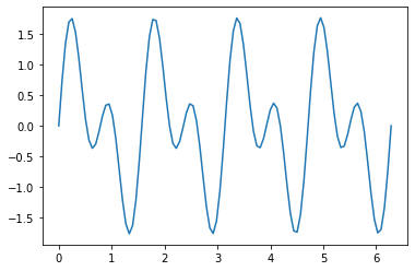

the function in frequency space typically has real and imaginary components.

fhat = fft(f)
fig, ax = plt.subplots(1,3, figsize=(12,4))
ax[0].plot(np.abs(fhat))
ax[0].set_title("abs")

ax[1].plot(np.real(fhat))
ax[1].set_title("real")

ax[2].plot(np.imag(fhat))
ax[2].set_title("complex")
plt.show()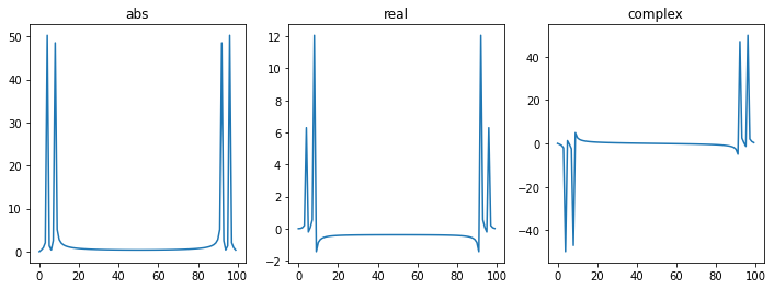

real-valued signals should have anti-symmetric complex components and symmetric real components.

f2 = ifft(fhat)
plt.plot(np.real(f2))
plt.show()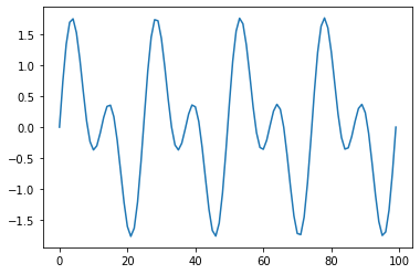

Fourier transforms can reveal a variety of useful information and have many useful properties. One of which is that convolutions in the time/spatial domain become pointwise multiplication in the frequency domain.

h = f \ast g \Leftrightarrow \hat{h} = \hat{f} \hat{g}

(6)

This means that circulant matrices and their inverses can be applied in $O(N \log N)$ time using the FFT.

def apply_circulant(c, x):
    """
    apply circulant matrix with first row c to a vector x
    
    y = C x
    """
    c_hat = fft(c)
    x_hat = fft(x)
    y_hat = c_hat * x_hat
    return ifft(y_hat)

N = 100
c = np.random.randn(N)
A = la.circulant(c)

x = np.random.randn(N)

%time y1 = A @ x
%time y2 = apply_circulant(c, x)

la.norm(y1 - y2)

CPU times: user 32 µs, sys: 3 µs, total: 35 µs
Wall time: 38.1 µs
CPU times: user 496 µs, sys: 0 ns, total: 496 µs
Wall time: 452 µs

3.7281796402185724e-14

def apply_circulant_inv(c, x):
    """
    apply inverse of circulant matrix with first row c to a vector x
    
    y = C^{-1} x
    """
    c_hat = fft(c)
    x_hat = fft(x)
    y_hat = x_hat / c_hat
    return ifft(y_hat)

N = 100
c = np.random.randn(N)
A = la.circulant(c)

x = np.random.randn(N)
b = A @ x

%time y1 = la.solve_circulant(c, x)
%time y2 = apply_circulant_inv(c, x)

la.norm(y1 - y2)

CPU times: user 1.04 ms, sys: 5 µs, total: 1.05 ms
Wall time: 1.15 ms
CPU times: user 1.17 ms, sys: 11 µs, total: 1.18 ms
Wall time: 880 µs

3.55434477453188e-15

Exercise 1¶

Create a plot that demonstrates the asymptotic scaling of the FFT is $O(N \log N)$

## Your code here

Exercise 2¶

Let $C$ be a circulant matrix.

Given that the inverse of a circulant matrix can also be applied using a Fourier transform, is $C^{-1}$ also a circulant matrix?

Write a function to compute the inverse of $C$ .

## Your code here

Higher Dimensions¶

In 2 dimensions, you can use scipy’s fft2 and ifft2 for 2-dimensional signals such as images. For an $m \times n$ image, the time complexity is $O(mn \log(mn))$

For general image processing, you may find it useful to install scikit-image

(pycourse) conda install scikit-image

Sparse Convolutions¶

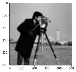
In image processing, you may often encounter sparse convolutions, particularly convolutions that are very localized (e.g. only the first few entries of the firs row c are nonzero). One example is that many camera lenses cause a slight blur which mixes light from nearby sources. In deep learning, these sparse convolutions have been very effective in image processing tasks. Perhaps the simplest explanation of why learning parameters for a convolution is a good idea in this situation is that convolutions are translation invariant allowing the neural net to learn regardless of where a target appears on an image.

In this case, we typically think of convolutions as $k\times k$ patches which slide over a 2-dimensional image.

The time complexity of applying this convolution using standard for-loops to a $m\times n$ image is $O(k^2 mn)$ , which is typically faster than using a Fourier transform. GPUs are also very good at this sort of operation.

import skimage

img = skimage.data.camera()
plt.imshow(img, cmap=plt.cm.gray)
plt.show()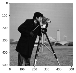

from numba import njit

@njit
def apply_convolution_2d(img, c):
    m, n = img.shape
    k1, k2 = c.shape
    img2 = np.zeros((m-k1, n-k2))
    for i in range(m-k1):
        for j in range(n-k2):
            for i1 in range(k1):
                for j1 in range(k2):
                    img2[i,j] = img2[i,j] + img[i+i1, j+j1] * c[i1, j1]
    return img2

c = np.ones((10,10)) / 100 # local averageing operator
%time img2 = apply_convolution_2d(img, c)

plt.imshow(img2, cmap=plt.cm.gray)
plt.show()

CPU times: user 88.6 ms, sys: 0 ns, total: 88.6 ms
Wall time: 89.4 ms

If you’re using this sort of convolution in PyTorch, you can use torch.nn.Conv2d or torch.conv2d

import torch

conv = torch.nn.Conv2d(1, 1, (3,3)) # 3 x 3 convolution

c = torch.Tensor(np.ones((1,1,10,10)) / 100)
imgt = torch.Tensor(img).reshape(1,1,*img.shape) # add batch and channel dimension

%time imgt2 = torch.conv2d(imgt, c)

CPU times: user 42.4 ms, sys: 13.7 ms, total: 56.2 ms
Wall time: 14.8 ms

img2 = imgt2.numpy()
img2 = img2[0,0,:,:]

plt.imshow(img2, cmap=plt.cm.gray)
plt.show()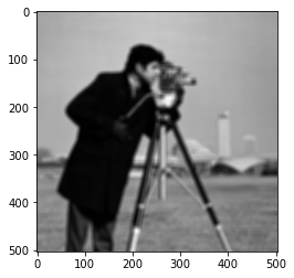

Discrete Cosine Transform (DCT)¶

One of the potential annoyances with Fourier transforms is that even with real-valued signals they produce complex output. If you want to stick to real output with a similar interpretation, you can use the Discrete Cosine Transform (DCT) or Discrete Sine Transform (DST). Both are implemented in Scipy.

Scipy DCT

from scipy.fft import dct, idct

x = np.linspace(0, 2*np.pi, 100)
f = np.sin(4*x) + np.sin(8*x)

fig, ax = plt.subplots(1, 2, figsize=(10, 5))
ax[0].plot(x, f)
ax[0].set_title("signal")

fhat = dct(f)
ax[1].plot(fhat)
ax[1].set_title("dct")
plt.show()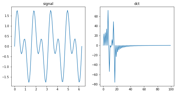

x = np.linspace(0, 2*np.pi, 100, endpoint=False)
f = np.cos(4*x) + np.cos(8*x)

fig, ax = plt.subplots(1, 2, figsize=(10, 5))
ax[0].plot(x, f)
ax[0].set_title("signal")

fhat = dct(f)
ax[1].plot(fhat)
ax[1].set_title("dct")
plt.show()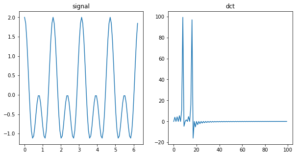

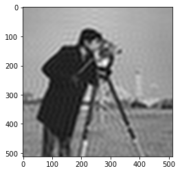
The DCT can also be used for a simple method of image compression - you can simply remove the high frequency componenents of an image and retain most of the large structure while losing some detail.

from scipy import ndimage
from scipy.fft import dctn, idctn
import skimage

img = skimage.data.camera()
plt.imshow(img, cmap=plt.cm.gray)
plt.show()

ihat = dctn(img)
plt.imshow(np.log(np.abs(ihat)))
plt.show()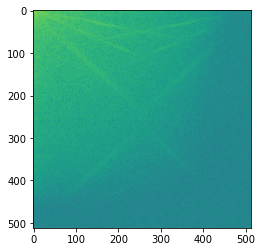

Now, we’ll cut out the highest-frequency DCT coefficients.

m, n = ihat.shape
ihat2 = ihat[:m//2, :n//2]
img2 = idctn(ihat2)
plt.imshow(img2, cmap=plt.cm.gray)
plt.show()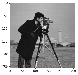

alternatively, we can make the image the original size by just setting the high-frequency DCT coefficients to 0.

ihat2 = np.zeros_like(ihat)
ihat2[:m//2, :n//2] = ihat[:m//2, :n//2]
img2 = idctn(ihat2)
plt.imshow(img2, cmap=plt.cm.gray)
plt.show()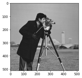

Now, let’s really compress the image...

ihat2 = np.zeros_like(ihat)
ihat2[:m//10, :n//10] = ihat[:m//10, :n//10]
img2 = idctn(ihat2)
plt.imshow(img2, cmap=plt.cm.gray)
plt.show()