Linear Algebra
Linear Algebra is the fundamental building block in scientific computing. Why? Even if we are dealing with complicated functions, we can always deal with approximations. If we want to understand a function near a point (sample), the simplest approximation is the constant function, which says the function is the same everywhere. This isn’t very interesting. The next level of approximation is a linear approximation, where we model the rate of change near that point. This is much more useful, even if it isn’t exact, and opens up the possibility of saying all kinds of things about the system that we’re studying.
In other words, you can do a lot with degree-1 Taylor series.
Let’s first recall some definitions from your mathematics classes:
A vector space over a field consists of a set of vectors which are related by addition and scalar multiplication
implies (addition)
implies
These operations are associative and commutative, etc. Usually what makes things interesting is the existence of a linear map.
A linear map is a map from one vector space () to another (, over the same field ) which satisfies
Matrices encode a linear map when we have chosen bases for both and .
In scientific computing the field is typically either the real numbers or complex numbers (but remember we use floating point arithmetic)
We will also deal with finite dimensional vector spaces. Sometimes these are explicitly vectors in Euclidean space (e.g. in computational geometry), but more often are some sort of function space.
Householder Notation
Householder notations is standard in numerical linear algebra:
scalars (elements of ) are denoted with lower-case Greek letters
vectors are denoted with lower-case Latin letters
matrices are denoted with capital letters (Latin or Greek), such as
This was introduced by Householder (see his book “Theory of Matrices in Numerical Analysis”, or the modern text “Matrix Computations” by Golub and Van Loan).
What Do we Compute?
basic operations - e.g. compute where
solving linear systems - find where .
matrix analysis - understand the action of the matrix via eigenvalues, SVD, etc.
Some Places where Linear Algebra Appears
Linear regression (example of linear system)
Principal components analysis (example of matrix analysis)
Solving ODE/PDE (depending on details, involves basic operations and solving linear systems)
Data Visualization (often use matrix analysis)
Optimization (gradient descent uses basic operations, Newton’s method solves a linear system)
Imaging - (basic operations, solving systems, some matrix analysis)
And the list goes on.
Example: Diffusion
One example where linear algebra appears is in measuring the strength of a signal at several sources from receivers. Consider a simplified problem where we have several points that emit some pollutant. We aren’t able to measure this pollutant directly at the sources. This can happen for a variety of reasons, such as:
The pollutant is completely inaccessible (e.g. far underwater)
We’re not able to get close for political reasons (people responsible won’t cooperate)
It is much cheaper to measure from other locations where we already have equipment
And so on. This problem is related to a variety of other problems in modeling heat or electromagnetic or acoustic signals, and is useful in imaging/remote sensing. We’ll denote the source locations with , and the receiver locations with . We’ll put these in a 2-dimensional plane
%matplotlib inline

import numpy as np
import matplotlib.pyplot as plt
nx = 3
ny = 3
np.random.seed(0)
x = np.random.rand(nx, 2)
y = np.random.rand(ny, 2)
plt.scatter(x[:,0], x[:,1], label='source')
plt.scatter(y[:,0], y[:,1], label='receiver')
plt.legend()
plt.show()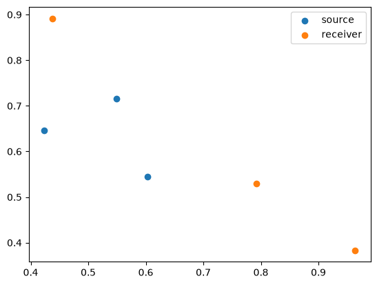
Each source emits the pollutant at rate . We represent this with a vector, where f[i] is the pollutant emitted by source i.
f = np.random.rand(nx)
f
array([0.56804456, 0.92559664, 0.07103606])We’ll assume the pollutant spreads via diffusion. What follows next might look familiar if you have taken some Physics classes before. If not, don’t worry - the basic idea is that pollution spreads out evenly from each source. As we get further away from the source, the pollution becomes less concentrated because it is spread out over a larger area. The function that tells us the concentration of a unit of pollution emitted by the source some distance away is called the Greens function.
Let denote the strength of the pollutant as a function in the 2-dimensional plane. This means that diffusion obeys the PDE
where is the laplacian, and is a dirac delta. We’re just going to measure the pollutant at the points , where the receivers are located. The amount of pollutant at receiver from source is
(this is the Green’s function for ). Because the total amount of pollution at each reciever is the sum of the pollution from each source measured at that receiver, we can write
where p[j] is the pollution at y[j], f[i] is the rate of pollution at source x[i], and G[j,i] is
G = np.empty((ny, nx), dtype=np.float64)
for i in range(nx):      # source
    for j in range(ny):  # receiver
        G[j,i] = -1.0/(2*np.pi) * np.log(np.linalg.norm(x[i] - y[j]))

G
array([[0.2493779 , 0.15224308, 0.22302595],
[0.10068884, 0.14768804, 0.08119219],
[0.18840228, 0.26461807, 0.15141249]])Now, we can calculate the concentration of pollution at the receivers using matrix-vector multipication
p = G @ f
p
array([0.29841632, 0.19966288, 0.36270623])However, the point is that we want to solve the inverse problem, which is to determine how much each source is polluting from our measurements at the receivers. In words, we want to find so that for some known .
If you were to write down the solution, you would find . However, you should never explicilty invert a matrix on a computer, because you often run into inaccuracy due to floating point representation error. For now, we’ll use np.linalg.solve
f2 = np.linalg.solve(G, p)
np.linalg.norm(f2 - f)np.float64(3.416972895534106e-14)G @ f2 - parray([0., 0., 0.])We see that the vector we solved for (f2) is very close to the true solution of f, and is close to machine precision.
We are able to accurately obtain the rates at which the sources release pollution based on measurements from some randomly placed sensors.
Linear Algebra In NumPy
Basic Operations
Vectors and matrices in NumPy are represented using np.ndarray, which we have seen already. Here is a review:
n = 3 # dimension of vector space
a, b = 1.5, 2.0 # scalars
x, y = np.random.rand(n), np.random.rand(n)

a*x + b*y # scalar multiplication and vector addition
array([1.68700745, 1.77035189, 3.20616645])m = 4 # dimension of target vector space
A = np.random.randn(m, n) # random linear transformation
z = A @ (a*x + b*y)
z # imagearray([ 0.98960871, -0.02812151, -3.75157541, 3.47067757])z2 = a * A @ x + b * A @ y
z2array([ 0.98960871, -0.02812151, -3.75157541, 3.47067757])z - z2 # difference of image computed in two waysarray([ 0.00000000e+00, -1.70002901e-16, 0.00000000e+00, -8.88178420e-16])k = 3
B = np.random.randn(k, m) # new linear map
z = (B @ A) @ x
z2 = B @ (A @ x)
z - z2array([-1.24900090e-16, 0.00000000e+00, 2.22044605e-16])Solving Linear Systems
Recall from our example that for numerical reasons, you should never invert a matrix to solve a linear system. Let’s see an example where we solve A @ x = b for x
import numpy.linalg as la
import time
n = 1000
A = np.random.randn(n,n)
x = np.random.rand(n)
b = A @ xt0 = time.time()
Ainv = la.inv(A) # use inversion
x2 = Ainv @ b
t1 = time.time()
print("{} sec.".format(t1 - t0))
la.norm(x - x2)0.022307872772216797 sec.
np.float64(4.1651748070961266e-11)t0 = time.time()
x2 = la.solve(A, b) # use solve function
t1 = time.time()
print("{} sec.".format(t1 - t0))
la.norm(x - x2)0.011479854583740234 sec.
np.float64(4.264671197622496e-12)We see that you will get a more precise answer, and faster when using solve instead of a matrix inverse.
If we want to do a least squares solve:
We can use lstsq. For full-rank (square) matrices, this is equivalent to solve.
x1 = la.solve(A, b)
x2 = la.lstsq(A, b, rcond=None)[0]
la.norm(x1 - x2)np.float64(6.964575844777663e-12)lstsq can also be used with over-and under determined linear systems
m = 1000
n = 500
A = np.random.randn(m, n)
x = np.random.rand(n)
b = A @ x
x2 = la.lstsq(A, b, rcond=None)[0]
la.norm(x - x2)np.float64(5.229269775919361e-14)in the above case, we are able to solve the system exactly because b in in the image of A
m = 500
n = 1000
A = np.random.randn(m, n)
x = np.random.rand(n)
b = A @ x
x2 = la.lstsq(A, b, rcond=None)[0]
la.norm(x - x2)np.float64(12.784556981877792)in the above case, there are many possiblities for x where A*x = b, so we find the smallest-norm solution
SciPy Linear Algebra
We’re now going to switch gears and start using scipy.linalg instead of numpy.linalg. From the user’s point of view, there isn’t really any difference, except scipy.linalg has all the same functions as numpy.linalg as well as additional functions. The call signatures are essentially the same, but there are sometimes different implementations under the hood.
SciPy is built on top of the NumPy ndarray data type, so it is fully interoperable. For example:
import scipy as sp
import scipy.linalg as sla
n = 1000
A = np.random.randn(n,n)
x = np.random.rand(n)
b = A @ x
x1 = la.solve(A, b) # numpy
x2 = sla.solve(A, b) # scipy
la.norm(x1 - x2)np.float64(0.0)We’ll just import scipy.linalg into the la namespace, replacing numpy.linalg
import scipy.linalg as laMatrix Factorizations
A matrix factorization or matrix decomposition writes a matrix as the product of matrices , where the matrices in the product typically have some special structure.
Here are some examples:
Diagonal matrices - easy to apply and solve linear systems
Triangular matrices (upper or lower) - fast to solve linear systems
Orthonormal matrices: orthogonal means (pseudoinverse)
Permutation matrices: sparse orthonormal matrices
Most of the matrix factorizations we will see run in time for a matrix , or for a matrix .
If you want to get really in-depth into how to compute matrix factorizations, take a numerical linear algebra course. We’ll get them treating scipy as a black box (meaning we don’t look inside).
LU decomposition
The first type of factorization we’ll look at is a decomposition, where is lower-triangular and is upper triangular. For numerical stability, this is often computed with a pivoting strategy, which means there is also row or column permutation matrix .
n = 1000
A = np.random.randn(n, n)
x = np.random.rand(n)
b = A @ x

P, L, U = la.lu(A)
la.norm(P @ L @ U - A)np.float64(2.7375882280132696e-12)The nice thing about triangular matrices is that they can solve linear systems in time, instead of time for general matrices, using the forward or backward substitution algorithms. There is a special function solve_triangular for this reason:
y = L @ x
x2 = la.solve_triangular(L, y, lower=True)
la.norm(x2 - x)4.610892733204046e-13We can replicate the functionality of solve using an LU factorization, using the expression
def my_solve(A, b):
    """
    solve A * x = b for x

    use LU decomposition
    """
    P, L, U = la.lu(A)
    x = la.solve_triangular(
            U,
            la.solve_triangular(
                L,
                P.T @ b,
                lower=True
            ),
            lower=False
        )
    return x
b = A @ x
x2 = my_solve(A, b)
la.norm(x - x2)5.545337890205843e-11Exercise
Use the
timemodule to perform an experiment to verify thatsolve_triangulartakes time. Hint: take LU decompositions of random matrices to get triangular factors of different sizes.
## Your code hereNotebook Cell
import time
tlist = list()
n  = np.logspace(0,np.log10(1000), num=100)
n = np.int64(np.round(n))

for i in n:
    A = np.random.randn(i, i)
    x = np.random.rand(i)
    b = A @ x
    P, L, U = la.lu(A)
    y = L @ x

    #Time for solve_triangular
    t0Tri = time.time()
    la.solve_triangular(L, y, lower=True)
    t1Tri = time.time()
    timeTri = t1Tri-t0Tri
    timeTri
    tlist.append(timeTri)

plt.plot(log(n),tlist, label='time vs log(n)')
plt.xlabel("n (in log) ")
plt.ylabel("Time")
plt.show()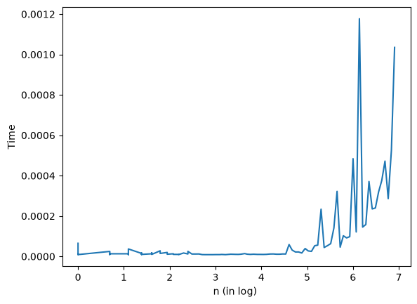
Suppose is , so the factorization above takes time. What is a big-O expression for the time to run
my_solveon ?
Notebook Cell
The big-O expression for the time to run my_solve on A is O(n^3) + O(n^2). LU factorization takes O(n^3) and each inverse of a triangular matrix takes O(n^2), but two triangular matrices are still O(n^2), and then we sum them up since there is an order performing the algorithm not composed.
QR decomposition
The decomposition, , contains a matrix with orthonormal columns, and an upper triangular matrix . For stability reasons, column pivoting is often used which means there is often a permutation matrix and .
m = 1000
n = 500
A = np.random.randn(m, n)

Q, R = la.qr(A, mode='economic') # no pivoting
la.norm(Q @ R - A)np.float64(8.243087056689126e-13)Q.shape, R.shape((1000, 500), (500, 500))Q, R, P = la.qr(A, pivoting=True) # pivoting
la.norm((Q @ R) - A[:,P])np.float64(8.002355261400986e-13)The QR factorization is used for least-squares solutions, because Q @ Q.T projects a vector onto the subspace spanned by the matrix A
def my_lstsq(A, b):
    """
    least squares solution ||b - A*x||

    Uses QR decomposition
    """
    Q, R = la.qr(A, mode='economic')
    x = la.solve_triangular(R, Q.T @ b, lower=False)
    return x
x = np.random.rand(n)
b = A @ x
x1 = la.lstsq(A, b)[0]
x2 = my_lstsq(A, b)
la.norm(x1 - x2)5.244247957288521e-14Excercise
Suppose is a matrix, and that the factorization takes time. What is the time to run my_lstsq using in big-O notation?
The computational complexity of QR factorization is , and the matirx-vector multiplication "" costs . Then solving has the cost of solving a triangular system . Thus, the overall computational complexity of my_lstsq is () or just (because we usually omit the lower orders).
Eigenvalue Decompositions
A vector is an eigenvector of with eigenvalue if . An eigenvalue decomposition is a decomposition where is a diagonal matrix. We can compute such a decomposition using eig:
n = 1000
A = np.random.randn(n, n)
Lam, X = la.eig(A)
columns of X are eigenvectors, and eigenvalues are diagonal entries of Lam
x = X[:,0]
la.norm(A @ x - Lam[0] * x)3.8400462682364843e-13When A is symmetric (or hermitian), there exists and orthonormal basis where every basis element is an eigenvector. In this case, we can write . There is a special function eigh for such a situation.
A = np.random.randn(n,n)
A = A + A.T # make symmetric
Lam, U = la.eigh(A)
x = U[:,0]
la.norm(A @ x - Lam[0] * x)3.2993189238553773e-13la.norm(U @ U.T - np.eye(n))np.float64(2.857495078064133e-12)Computing eigenvector decompositions takes time for a matrix.
Exercises
Both
eigandeightake time. Which is faster in practice on a symmetric matrix? Do they produce the same answer on the same symmetric matrix?
As shown in the figure, eigh is much faster than eig in practice. We checked the eigenvalues produced by both methods (eigenvalues of eigh are sorted), they produced the same answer.
Write a function that solves a linear system with a symmetric matrix using the Eigenvalue decomposition. Is this function faster or slower than using LU in
my_solve?
As shown in the figure, my_solve is faster than eigh in practice.
## Your code here
Notebook Cell
## Your code here
'''
1. Compare the speed and difference of eig & eigh
'''
n = np.logspace(0,np.log10(1000), num=100)
n = np.int64(np.round(n))
teig=list()
teigh=list()
valdiff = list()
for i in n:
    A = np.random.randn(i,i)
    A = A + A.T
    t0eig = time.time()
    Lam1, X = la.eig(A)
    t1eig = time.time()
    teigdiff = t1eig-t0eig
    teig.append(teigdiff)

    t0eigh = time.time()
    Lam2, U = la.eigh(A)
    t1eigh = time.time()
    teighdiff = t1eigh-t0eigh
    teigh.append(teighdiff)

    valdiff.append(np.max(np.abs(np.sort(Lam1) - np.sort(Lam2))))
Notebook Cell
'''
1. Time comparison
'''
plt.plot(np.log(n),teig, label='eig')
plt.plot(np.log(n),teigh, label='eigh')
plt.xlabel("n (in log) ")
plt.ylabel("Time")
plt.legend(loc='best')
plt.show()

'''
1. Difference
'''
np.max(valdiff)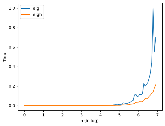
np.float64(1.5774048733874224e-12)Notebook Cell
'''
2. Compare the speed of EVD v.s. LU when solving linear systems
'''
def solve_eigh(A, b):
    Lam, U = la.eigh(A)
    Ainv = U@np.diag(1/Lam)@U.T
    x = Ainv@b
    return(x)


n = np.logspace(0,np.log10(1000), num=100)
n = np.int64(np.round(n))
tlu=list()
teigh=list()
valdiff = list()
for i in n:
    A = np.random.randn(i,i)
    A = A + A.T
    x = np.random.rand(i)
    b = A @ x
    t0lu = time.time()
    x1 = my_solve(A, b)
    t1lu = time.time()
    tludiff = t1lu-t0lu
    tlu.append(tludiff)

    t0eigh = time.time()
    x2 = solve_eigh(A,b)
    t1eigh = time.time()
    teighdiff = t1eigh-t0eigh
    teigh.append(teighdiff)
Notebook Cell
'''
2. Time comparison
'''
plt.plot(np.log(n),tlu, label='lu')
plt.plot(np.log(n),teigh, label='eigh')
plt.xlabel("n (in log) ")
plt.ylabel("Time")
plt.legend(loc='best')
plt.show()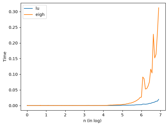
SVD
The singular value decomposition is an extremely useful practical and theoretical tool. We can decompose a matrix as , where is a matrix with orthonormal columns (called left singular vectors), is a matrix with orthonormal columns (called right singular vectors), and is a diagonal matrix with positive entries decreasing in magnitude (called singular values).
The top singular value solves the variational problem subject to , and describes the direction in which induces the largest change in maginitude in a vector. The next singular value is defined similarly on the subspaces orthogonal to and , and so on.
One way to visualize the action of a matrix is seeing how it maps the unit sphere. The image is an ellipsoid, and the right singular vectors give the directions of the axes, and the singular values give the lengths of these axes.
n = 2
A = np.random.randn(n,n)
U, S, Vt = la.svd(A)
theta = np.linspace(0, 2*np.pi, num=200, endpoint=True)
xx = np.vstack((np.cos(theta), np.sin(theta)))
yy = A @ xx
fig = plt.figure(figsize=(10,10))
ax = fig.add_subplot(111)
ax.plot(yy[0], yy[1])
ax.set_aspect('equal')
ax.scatter(S*U[0], S*U[1])
plt.show()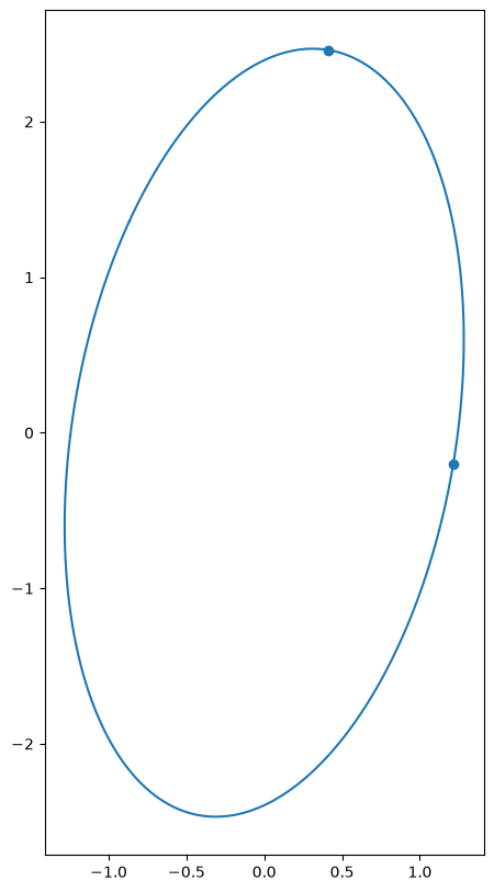
Exercises
Computing the SVD takes time for a matrix, just like all the other matrix factorizations we’ve seen. Make plots of the runtimes of
svd,eigh,eig,qrandluas we increase . Which is fastest in practice?
From the plot, we see that from slowest to fastest is: eig, svd, eigh, qr, lu. lu is fastest in practice.
Write a function that solves a linear system using the Singular Value Decomposition.
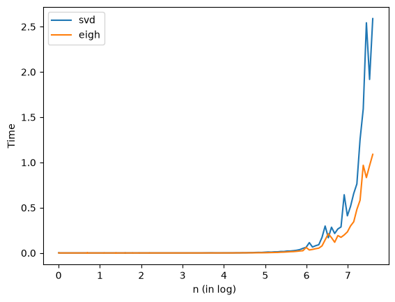
What is the SVD of a Hermitian (symmetric matrix)? Is
svdoreighfaster?
From the last figure, we can see that eigh is faster on a Hermitian.
## Your code here
Notebook Cell
'''
1. Time comparison of SVD, eig, eigh, QR, LU
'''
n = np.logspace(0,np.log10(1000), num=100)
n = np.int64(np.round(n))
tsvd=list()
teigh=list()
teig=list()
tqr=list()
tlu=list()

for i in n:
    A = np.random.randn(i,i)

    t0 = time.time()
    U, S, Vt = la.svd(A)
    t1 = time.time()
    tsvd.append(t1-t0)

    t0 = time.time()
    Lam, U = la.eig(A)
    t1 = time.time()
    teig.append(t1-t0)

    t0 = time.time()
    Lam, U = la.eigh(A)
    t1 = time.time()
    teigh.append(t1-t0)

    t0 = time.time()
    Q, R = la.qr(A, mode='economic') # no pivoting
    t1 = time.time()
    tqr.append(t1-t0)

    t0 = time.time()
    P, L, U = la.lu(A)
    t1 = time.time()
    tlu.append(t1-t0)
Notebook Cell
'''
1. Time comparison of SVD, eig, eigh, QR, LU
'''
plt.plot(np.log(n),teig, label='eig')
plt.plot(np.log(n),tsvd, label='svd')
plt.plot(np.log(n),teigh, label='eigh')
plt.plot(np.log(n),tqr, label='qr')
plt.plot(np.log(n),tlu, label='lu')
plt.xlabel("n (in log) ")
plt.ylabel("Time")
plt.legend(loc='best')
plt.show()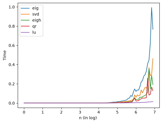
Notebook Cell
'''
2. Define a function that solves a linear system using SVD
'''
def solve_svd(A, b):
    U, S, Vt = la.svd(A)
    Ainv = U@np.diag(1/S)@Vt
    x = Ainv@b
    return(x)
Notebook Cell
'''
3. Compare svd and eigh on symmetric matrices
'''

n = np.logspace(0,np.log10(2000), num=100)
n = np.int64(np.round(n))
tsvd=list()
teigh=list()

for i in n:
    A = np.random.randn(i,i)
    A = A + A.T
    t0 = time.time()
    U, S, Vt = la.svd(A)
    t1 = time.time()
    tsvd.append(t1-t0)

    t0 = time.time()
    Lam, U = la.eigh(A)
    t1 = time.time()
    teigh.append(t1-t0)
Notebook Cell
plt.plot(np.log(n),tsvd, label='svd')
plt.plot(np.log(n),teigh, label='eigh')
plt.xlabel("n (in log) ")
plt.ylabel("Time")
plt.legend(loc='best')
plt.show()