Monte Carlo Methods - Scientific Computing with Python

Monte carlo methods are a class of methods that use randomness to make it easier to solve deterministic problems. Specifally, we wish to compute integrals of the form

\int f(x) p(x) dx

(1)

where $p$ is a probability density, i.e. a non-negative “function” that integrates to 1.

The idea of Monte-Carlo, is to observe that, if $X$ is a random variable distributed according to $p$ , then

\mathbb{E}[f(X)] = \int f(x) p(x)dx

(2)

We can then estimate the expectation using the law of large numbers. We suppose that $X_1,\;X_2,\;X_3,\;\ldots$ are all random variables distributed according to $p$ . Then the law of large numbers gives that

\frac1n \sum_{i=1}^n f(X_i) \to \mathbb{E}[f(X_1)]=\int f(x)p(x)dx.

(3)

A classical example of this, is to compute the area of the unit circle ( $\pi$ )

\pi=\int_{D_1} 1 dx = \int_{[-1,1]\times[-1,1]} \chi_{D_1}(x) dx = 4 \mathbb{E[\chi_{D_1}(U_{[-1,1]\times[-1,1]})}],

(4)

where $\chi_{D_1}$ is the indicator function of the unit disk.

import numpy as np
import scipy
import matplotlib.pyplot as plt

n = 1000;

xs = 2*np.random.rand(2,n)-1
plt.scatter(xs[0,:],xs[1,:])

ids = np.linalg.norm(xs,axis=0)<1
plt.scatter(xs[0,ids],xs[1,ids])

fn = 4*sum(ids)/n
'estimate = {}'.format(fn)
'error = {}'.format(fn-np.pi)

'error = 0.04240734641020705'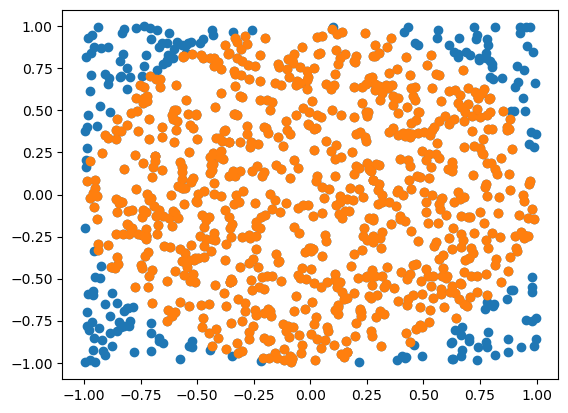

Let’s look at how this converges with $n$

ns = np.int32(np.logspace(0,6,100))
errs = []
for n in ns:
    xs = 2*np.random.rand(2,n)-1
    ids = np.linalg.norm(xs,axis=0)<1
    errs.append((4*sum(ids)/n)-np.pi)
    
plt.loglog(ns,np.abs(errs),'o-')
plt.loglog(ns,1/np.sqrt(ns),'-')
plt.xlabel('n')
plt.ylabel('Error')
plt.show()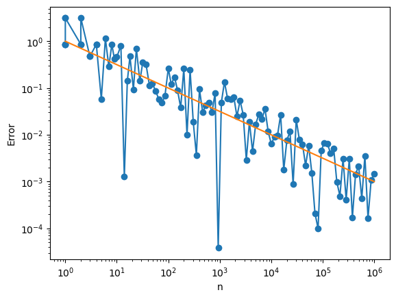

Let’s look at why the error is decaying like $\frac{1}{\sqrt{n}}$ . Let’s let the estimator

\hat{f}_n = \frac1n \sum_n f(X_i).

(5)

The variance of $\hat{f}_n$ is

\mathbb{E}\left[(\hat{f}_n-\hat{E}[f(X)])^2\right] = \frac{1}{n^2} \mathbb{E}\left[\left(\sum_{i=1}^n f(X_i)-\mathbb{E}[\hat{f}(X)]\right)^2\right] = \frac{1}{n^2} \sum_{i,j} \mathbb{E}\left[\left(f(X_i)-\mathbb{E}[\hat{f}(X)]\right)\left(f(X_j)-\hat{E}[f(X)]\right)\right].

(6)

If we rearrange this a bit, we get

\mathbb{E}\left[(\hat{f}_n-\hat{E}[f(X)])^2\right] =\frac{1}{n^2} \left(\sum_{i} \mathbb{E}\left[\left(f(X_1)-\mathbb{E}[\hat{f}(X)]\right)^2\right] +\sum_{i\neq j} \text{Cov}(f(X_i),(X_j)) \right)

(7)

Since the $X_i$ ’s are independent, $\text{Cov}(f(X_i),(X_j))=0$ well $i\neq j$ .

\mathbb{E}\left[(\hat{f}_n-\hat{E}[f(X)])^2\right] =\frac{1}{n} \mathbb{E}\left[\left(f(X_1)-\mathbb{E}[\hat{f}(X)]\right)^2\right].

(8)

If we take square root

\sqrt{\mathbb{E}\left[(\hat{f}_n-\hat{E}[f(X)])^2\right]} =\frac{1}{\sqrt{n}} \sqrt{\mathbb{E}\left[\left(f(X_1)-\mathbb{E}[\hat{f}(X)]\right)^2\right]},

(9)

we see that the average error will decay like $\frac{1}{\sqrt{n}}$ .

This one over square root $n$ error is universal in Monte Carlo. It is both the advantage and the curse of Monte Carlo.

Suppose we are trying to compute an integral in $d$ dimensions using a $p$ th order rule using $n$ points. The error is

O\left( \sqrt[d]{n}^{-p}\right) = O\left( n^{-p/d}\right),

(10)

which will be very slow when $d$ is large. This will be a lot smaller than the error of Monte Carlo when $d>2p$

O\left(n^{-1/2} \right).

(11)

Importance sampling¶

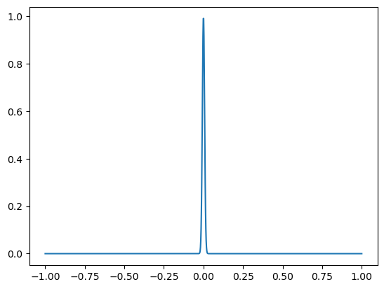
Suppose we want to compute the integral of a highly concentrated function

\int_{-\infty}^\infty e^{-10^4x^2} dx = \frac{\sqrt{\pi}}{10^4}

(12)

We shall truncate to the interval $[-1,1]$ , since the function is very small there.

f = lambda x: np.exp(-1e4*x*x)
xs = np.linspace(-1,1,1000)
plt.plot(xs,f(xs))
plt.show()


true_int = np.sqrt(np.pi)/100

ns = np.int32(np.logspace(0,5,20))
ntrial = 10
errs = []
for n in ns:
    errs_samp = np.zeros(ntrial)
    for k in range(ntrial):
        xs = 2*np.random.rand(1,n)-1
        errs_samp[k] = ((2*np.sum(f(xs))/n)-true_int)/true_int
        
    errs.append(np.mean(errs_samp))
    
plt.loglog(ns,np.abs(errs),'o-')
plt.loglog(ns,1/np.sqrt(ns),'-')
plt.xlabel('n')
plt.ylabel('Relative error')
plt.show()

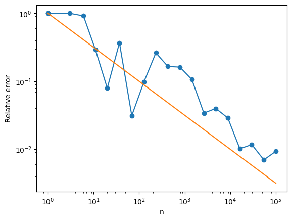
We can increase the accuracy, we should use Monte Carlo samples where $f$ is large. If the samples $X_i$ are drawn from the pobability distribution $p$ , then we compensate for this by

\int_{-\infty}^\infty f(x)dx = \int_{-\infty}^\infty \frac{f(x)}{p(x)} p(x)dx \approx \frac{1}{n} \sum_{i}\frac{f(x_i)}{p(x_i)}

(13)

We shall choose $p$ to be the density for a normal distrubtion: $p(x) = \frac{1}{\sqrt{2\pi\sigma^2}} \exp(-\frac{x^2}{2\sigma^2})$

for sigma in [1e-2,1e-1, 1]:
    p = lambda x: np.exp(-x*x/2/sigma/sigma)/np.sqrt(2*np.pi*sigma**2)
    errs_import = []
    for n in ns:
        errs_samp = np.zeros(ntrial)
        for k in range(ntrial):
            xs = sigma * np.random.randn(1,n)
            est = np.sum(f(xs)/p(xs)) / n
            errs_samp[k] = (est-true_int)/true_int
        errs_import.append(np.mean(errs_samp))

    plt.loglog(ns,np.abs(errs_import),'o-',label='sigma={}'.format(sigma))

plt.loglog(ns,np.abs(errs),'*--',label='uniform')    
plt.loglog(ns,1/np.sqrt(ns),':')
plt.xlabel('n')
plt.legend()
plt.ylabel('Relative error')
plt.show()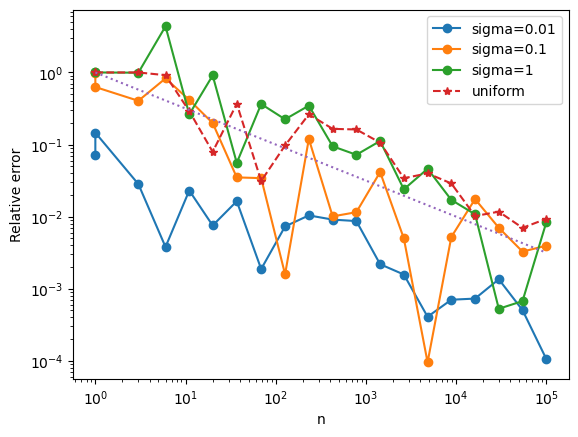

We see that concentrating the samples at the peak of the function significantly decreases the error. This method is called “importance sampling”.

Markov Chain Monte Carlo (MCMC)¶

Sometimes we wish to compute

\int f(x) p(x) dx

(14)

but we can’t directly sample from $p$ . The idea will be to choose our samples $X_i$ to be samples from a Markov chain. i.e. $X_{i+1}$ is randomly generated from $X_i$ . If we run it long enough, then the $X_i$ ’s will be distributed according to the stationary distribution of the Markov chain.

Our task is therefore to design a Markov chain whose stationary distribution is $p$ .

Metropolis-Hastings¶

We shall generate a sample $Y_{i+1}$ from $X_i$ . i.e. $Y_{i+1}=X_i + \Delta_i$ .

Then we set $X_{i+1}=Y_{i+1}$ with probability $\text{min}(p(Y_{i+1})/p(X_i),1)$ and set $X_{i+1}=X_i$ otherwise.

You can check that the stationary probability is $p$ .

Note that we don’t need the value of $p$ , we only need the ratio, so $p$ need not be normalized.

Let’s use this to compute

\int_{-\infty}^\infty x^2 Z^{-1}e^{-V(x)} dx,

(15)

where $V(x)=x^2$ and $Z=\int e^{-V(x)}$ . The corresponding $p(x) = Z^{-1} e^{-V(x)}$ .

Note that the samples are no longer independent. The covariance between samples will lower the effective number of samples, but the estimator will still converge.

def MC_step(x,p):
    delta = 0.1
    y = x + delta*np.random.randn()
    prob = min(p(y)/p(x),1)
    if np.random.rand() < prob:
        x = y
    return x

V = lambda x: x**4-x**2
p = lambda x: np.exp(-V(x))

nburn_in = 1000
x = 0
for i in range(nburn_in):
    x = MC_step(x,p)
    
nsample = 10000
xs = [x]
for i in range(nsample):
    x = MC_step(x,p)
    xs.append(x)

xs = np.array(xs)
sum(xs*xs)/nsample
plt.hist(xs,bins=50)
plt.show()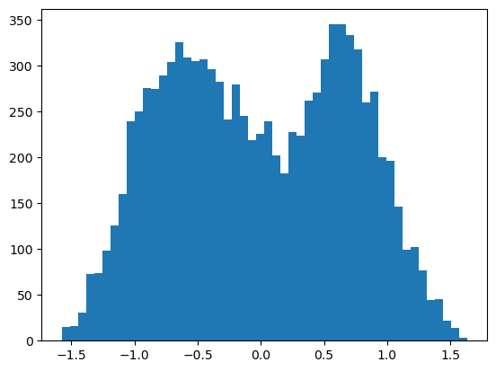

xx = np.linspace(-1.5,1.5,200)
plt.plot(xx,p(xx),'.')
kde = scipy.stats.gaussian_kde(xs)
plt.plot(xx,kde(xx))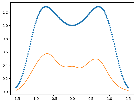

Such examples occur in statistical physics.