Scipy stats package - Scientific Computing with Python

A variety of functionality for dealing with random numbers can be found in the scipy.stats package.

import numpy as np
from scipy import stats
from scipy.stats import laplace, poisson
from scipy.stats import norm as normal
import matplotlib.pyplot as plt

Distributions¶

There are over 100 continuous (univariate) distributions and about 15 discrete distributions provided by scipy

To avoid confusion with a norm in linear algebra we’ll import stats.norm as normal

from scipy.stats import norm as normal

A normal distribution with mean $\mu$ and variance $\sigma^2$ has a probability density function

\frac{1}{\sigma \sqrt{2\pi}} e^{-(x-\mu)^2 / 2\sigma^2}

(1)

# bounds of the distribution accessed using fields a and b
normal.a, normal.b

(-inf, inf)

# mean and variance
normal.mean(), normal.var()

(0.0, 1.0)

# Cumulative distribution function (CDF)
x = np.linspace(-5,5,100)
y = normal.cdf(x)
plt.plot(x, y)
plt.title('Normal CDF');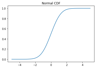

# Probability density function (PDF)
x = np.linspace(-5,5,100)
y = normal.pdf(x)
plt.plot(x, y)
plt.title('Normal PDF');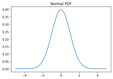

You can sample from a distribution using the rvs method (random variates)

X = normal.rvs(size=1000)
plt.hist(X);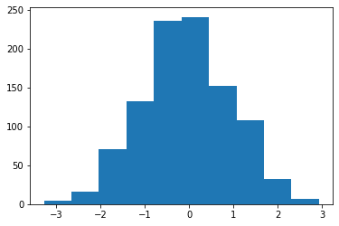

You can set a global random state using np.random.seed or by passing in a random_state argument to rvs

X = normal.rvs(size=1000, random_state=0)
plt.hist(X);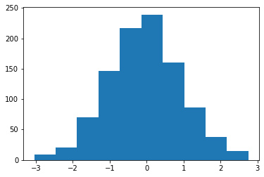

To shift and scale any distribution, you can use the loc and scale keyword arguments

X = normal.rvs(size=1000, random_state=0, loc=1.0, scale=0.5)
plt.hist(X);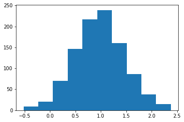

# Probability density function (PDF)
x = np.linspace(-5,5,100)
y = normal.pdf(x, loc=1.0, scale=0.5)
plt.plot(x, y)
plt.title('Normal PDF');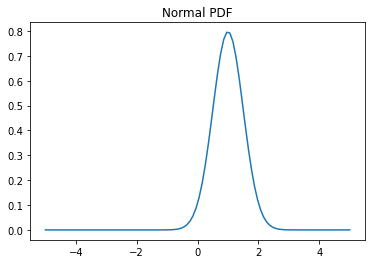

You can also “freeze” a distribution so you don’t need to keep passing in the parameters

dist = normal(loc=1.0, scale=0.5)
X = dist.rvs(size=1000, random_state=0)
plt.hist(X);

Example: The Laplace Distribution¶

We’ll review some of the methods we saw above on the Laplace distribution, which has a PDF

\frac{1}{2}e^{-|x|}

(2)

from scipy.stats import laplace

x = np.linspace(-5,5,100)
y = laplace.pdf(x)
plt.plot(x, y)
plt.title('Laplace PDF');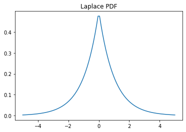

x = np.linspace(-5,5,100)
y = laplace.cdf(x)
plt.plot(x, y)
plt.title('Laplace CDF');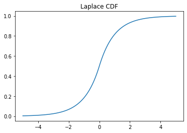

X = laplace.rvs(size=1000)
plt.hist(X);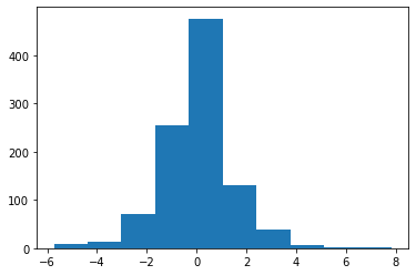

laplace.a, laplace.b

(-inf, inf)

laplace.mean(), laplace.var()

(0.0, 2.0)

Discrete Distributions¶

Discrete distributions have many of the same methods as continuous distributions. One notable difference is that they have a probability mass function (PMF) instead of a PDF.

We’ll look at the Poisson distribution as an example

from scipy.stats import poisson
dist = poisson(1) # parameter 1

dist.a, dist.b

(0, inf)

dist.mean(), dist.var()

(1.0, 1.0)

x = np.arange(10)
y = dist.pmf(x)
plt.scatter(x, y);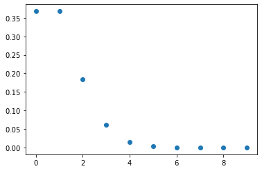

x = np.linspace(0,10, 100)
y = dist.cdf(x)
plt.plot(x, y);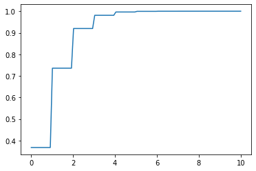

X = dist.rvs(size=1000)
plt.hist(X);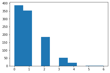

Fitting Parameters¶

You can fit distributions using maximum likelihood estimates

X = normal.rvs(size=100, random_state=0)

normal.fit_loc_scale(X)

(0.059808015534485, 1.0078822447165796)

Statistical Tests¶

You can also perform a variety of tests. A list of tests available in scipy available can be found here.

the t-test tests whether the mean of a sample differs significantly from the expected mean

stats.ttest_1samp(X, 0)

Ttest_1sampResult(statistic=0.5904283402851698, pvalue=0.5562489158694675)

The p-value is 0.56, so we would expect to see a sample that deviates from the expected mean at least this much in about 56% of experiments. If we’re doing a hypothesis test, we wouldn’t consider this significant unless the p-value were much smaller (e.g. 0.05)

If we want to test whether two samples could have come from the same distribution, we can use a Kolmogorov-Smirnov (KS) 2-sample test

X0 = normal.rvs(size=1000, random_state=0, loc=5)
X1 = normal.rvs(size=1000, random_state=2, loc=5)

stats.ks_2samp(X0, X1)

KstestResult(statistic=0.023, pvalue=0.9542189106778983)

We see that the two samples are very likely to come from the same distribution

X0 = normal.rvs(size=1000, random_state=0)
X1 = laplace.rvs(size=1000, random_state=2)

stats.ks_2samp(X0, X1)

KstestResult(statistic=0.056, pvalue=0.08689937254547132)

When we draw from a different distribution, the p-value is much smaller, indicating that the samples are less likely to have been drawn from the same distribution.

Kernel Density Estimation¶

We might also want to estimate a continuous PDF from samples, which can be accomplished using a Gaussian kernel density estimator (KDE)

X = np.hstack((laplace.rvs(size=100), normal.rvs(size=100, loc=5)))
plt.hist(X);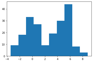

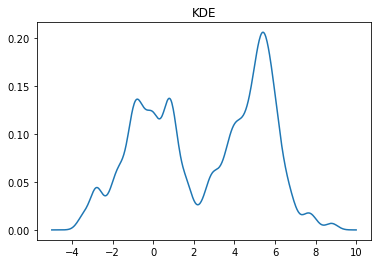
A KDE works by creating a function that is the sum of Gaussians centered at each data point. In Scipy this is implemented as an object which can be called like a function

kde = stats.gaussian_kde(X)
x = np.linspace(-5,10,500)
y = kde(x)
plt.plot(x, y)
plt.title("KDE");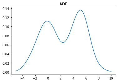

We can change the bandwidth of the Gaussians used in the KDE using the bw_method parameter. You can also pass a function that will set this algorithmically. In the above plot, we see that the peak on the left is a bit smoother than we would expect for the Laplace distribution. We can decrease the bandwidth parameter to make it look sharper:

kde = stats.gaussian_kde(X, bw_method=0.2)
x = np.linspace(-5,10,500)
y = kde(x)
plt.plot(x, y)
plt.title("KDE");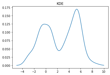

If we set the bandwidth too small, then the KDE will look a bit rough.

kde = stats.gaussian_kde(X, bw_method=0.1)
x = np.linspace(-5,10,500)
y = kde(x)
plt.plot(x, y)
plt.title("KDE");